We ran 32,000 simulated experiments across four common marketing scenarios to benchmark four leading open-source geo-experiment tools. Because we use synthetic data where the true campaign effect is known in advance, we can measure how well each tool recovers it.
These four tools are often treated as interchangeable, and they are not. Where they diverge — sharply, at times — is in how they handle uncertainty: how often their confidence intervals contain the true incremental effect, how often they declare winning results that aren't real (false positives), and how often they come back inconclusive when a real incremental effect exists (false negatives).
Every tool forces a tradeoff between those two mistakes, and the choice of tool becomes a choice about which one is more expensive for your business. That's the focus of this report.
We compared four leading open-source geographic-based experimentation tools — CausalPy, Google Matched Markets, Google Causal Impact, and Meta GeoLift — by running each one on thousands of simulated datasets where the true incremental campaign effect is known beforehand. Throughout this report, "effect" means this incremental lift — the sales a campaign genuinely causes, beyond what would have happened anyway.
In this study, every tool sees the same data, the same treatment and control markets, and is scored against the same ground truth. The only thing that differs is the tool being used for the analysis.
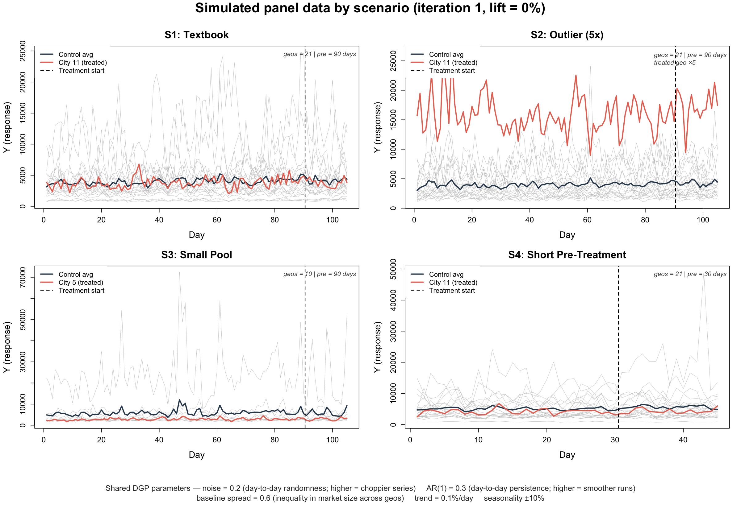
Each simulated dataset is daily sales across many markets, ending with a two-week test period. In that window, one market gets either a 7.5% incremental sales lift (to see whether each tool detects a real effect) or no lift at all (to see how often each tool declares a false win). Each market behaves like a real one: it has its own size, grows slowly over time, has good days and bad days of the week, and experiences random noise where a rough patch tends to bleed into the next day rather than resetting completely.
For the full methodology and technical details, see the Appendix.
We tested the tools across four scenarios. Each represents a real-world operating condition you'll meet in the course of running an experimentation program.
This is clean, well-behaved data with one treated geo and a diverse pool of 20 control markets.
The treated market is 5x larger than the median city in the control pool. In other words, what happens when your CMO insists on testing in New York?
There are only 9 control markets instead of 20, a common issue for companies operating in smaller markets.
This has 30 days of pre-treatment data instead of 90. Again, a common occurrence where business pressure forces a brand to launch an experiment before they have sufficient pre-experiment data.
Across these scenarios, no tool escaped the tradeoff between false positives and false negatives. The interesting question is which tradeoff each one made.
Every tool in this study forces a choice between two errors: false positives (declaring a winning experiment that isn't real) and false negatives (declaring an experiment inconclusive when a real incremental effect exists). No tool escapes the tradeoff. Which mistake is more expensive for your business is the question that should drive which tool you pick.
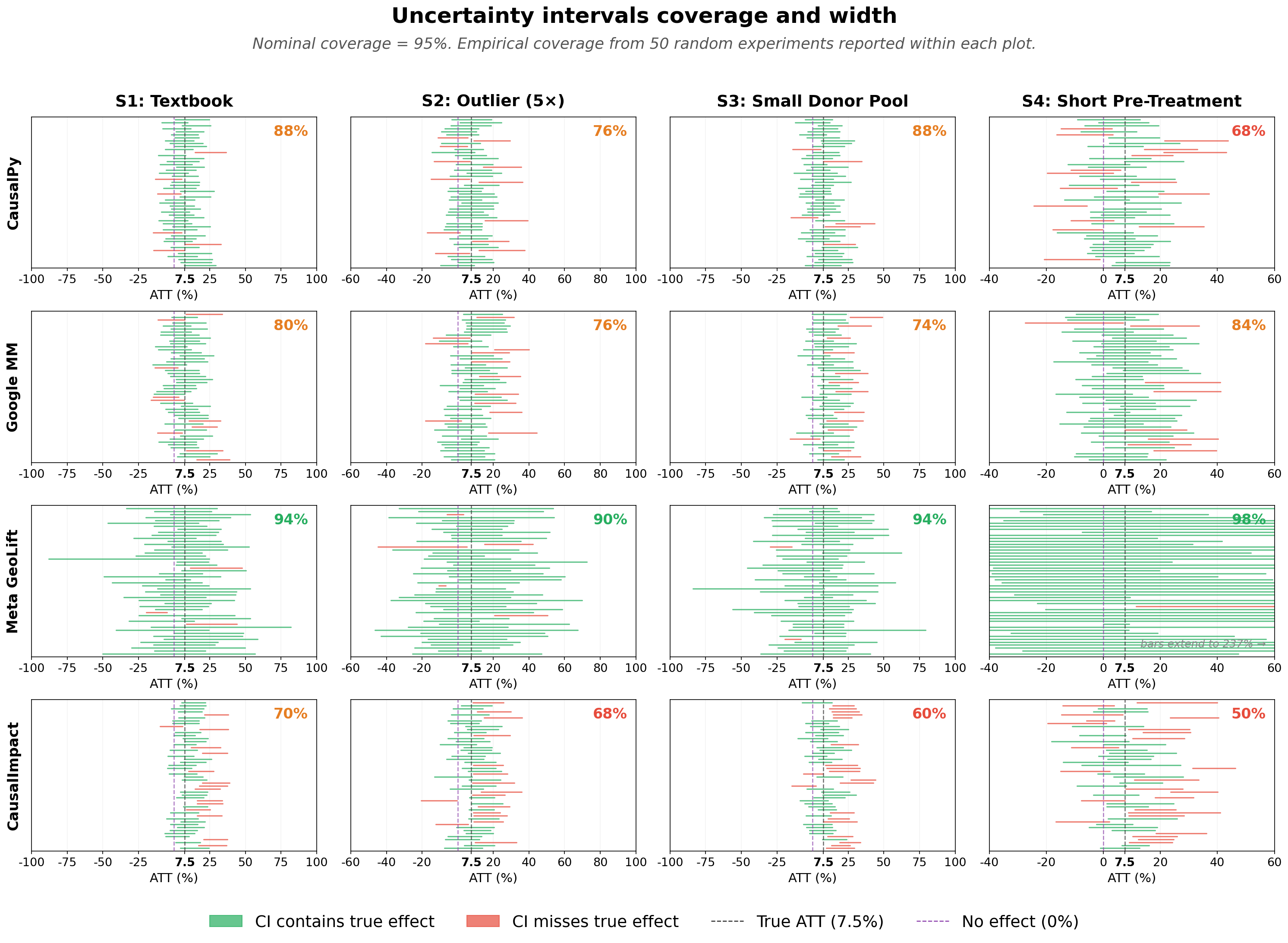
When a tool provides a confidence interval — for example, "the incremental lift is between 5.2% and 10.1% with 95% confidence" — that interval is supposed to contain the true answer 95% of the time. Keeping that promise comes at a cost. A tool can produce wide intervals that reliably contain the true lift. But if those intervals become so wide that they contain zero, the experiment can't declare a statistically significant effect, even when a real one exists.
On the other hand, a tool can produce tighter, more decisive intervals. But those intervals will miss the true incremental lift more often and generate more false alarms. No tool in this study escapes this tradeoff.
Meta GeoLift is the strongest performer on three of four metrics under consideration: its coverage is closest to the 95% target (92–95%), it has the lowest false positive rate (3–5%), and its point estimates are closest to the true incremental lift in most scenarios. The tradeoff is in its ability to detect real incremental effects, where Meta GeoLift's confidence intervals are wide enough such that they frequently contain both the true effect and zero at the same time. This conservatism can become a limitation for practitioners making decisions with output from the tool.
Causal Impact sits at the opposite end. Its intervals are narrow enough to exclude zero most of the time, which is why it declares a statistically significant lift more often than any other tool — flagging the real 7.5% effect in 52–66% of runs. But narrow intervals that confidently exclude zero also confidently exclude zero when they shouldn't. Causal Impact fires false alarms nearly 30% of the time, and its estimates carry a consistent positive bias that shifts the whole interval high — making campaigns look more effective than they are. Causal Impact is a decisive tool, but it is often confidently wrong.
Google MM and CausalPy sit in between, with coverage of 76–86% and false positive rates of 14–25%. Their confidence intervals are wide enough to avoid constant false alarms, but not so wide that every experiment ends inconclusively. The cost is that they under-deliver on the 95% coverage promise in both directions with more false positives than Meta GeoLift and less detection power than Causal Impact.
"The numbers above tell you what each tool's tradeoff actually is. With this context, picking among them becomes a business decision rather than just a statistical one."
The 30-day pre-treatment scenario (S4) delivers a highly practical finding: it reflects a situation many practitioners have faced, where leadership wants to move faster than the data allows.
With only 30 days of pre-treatment data, Meta GeoLift and Google MM hold up better than CausalPy and Causal Impact. Importantly, the pattern from Finding 1 doesn't ease under data scarcity — it sharpens. Conservative tools become even more conservative and yield more inconclusive experiments. Decisive tools produce more false reads that can mislead marketers.
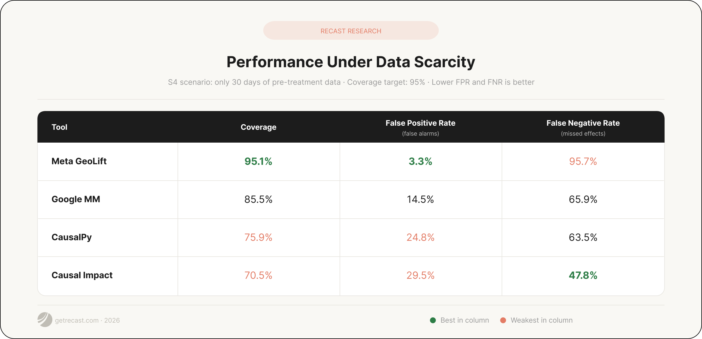
The practical takeaway: 30 days of pre-treatment data is insufficient for reliable inference with any of these tools. But if you're in that situation, Meta GeoLift and Google MM give you a more defensible result.
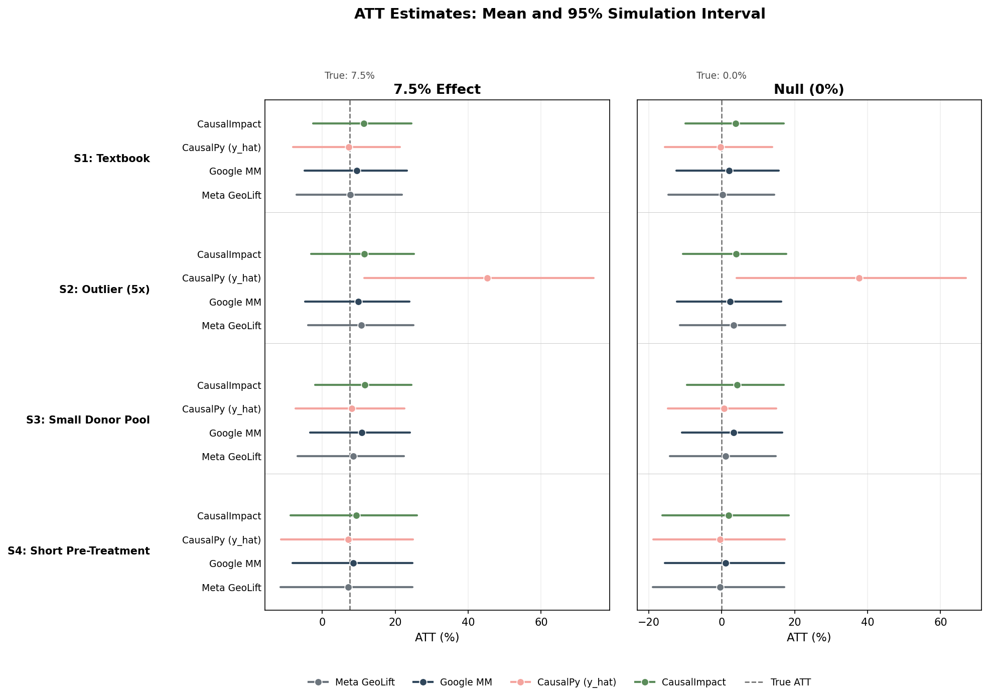
Across non-outlier scenarios, all four tools largely recover the true 7.5% lift within a few percentage points.
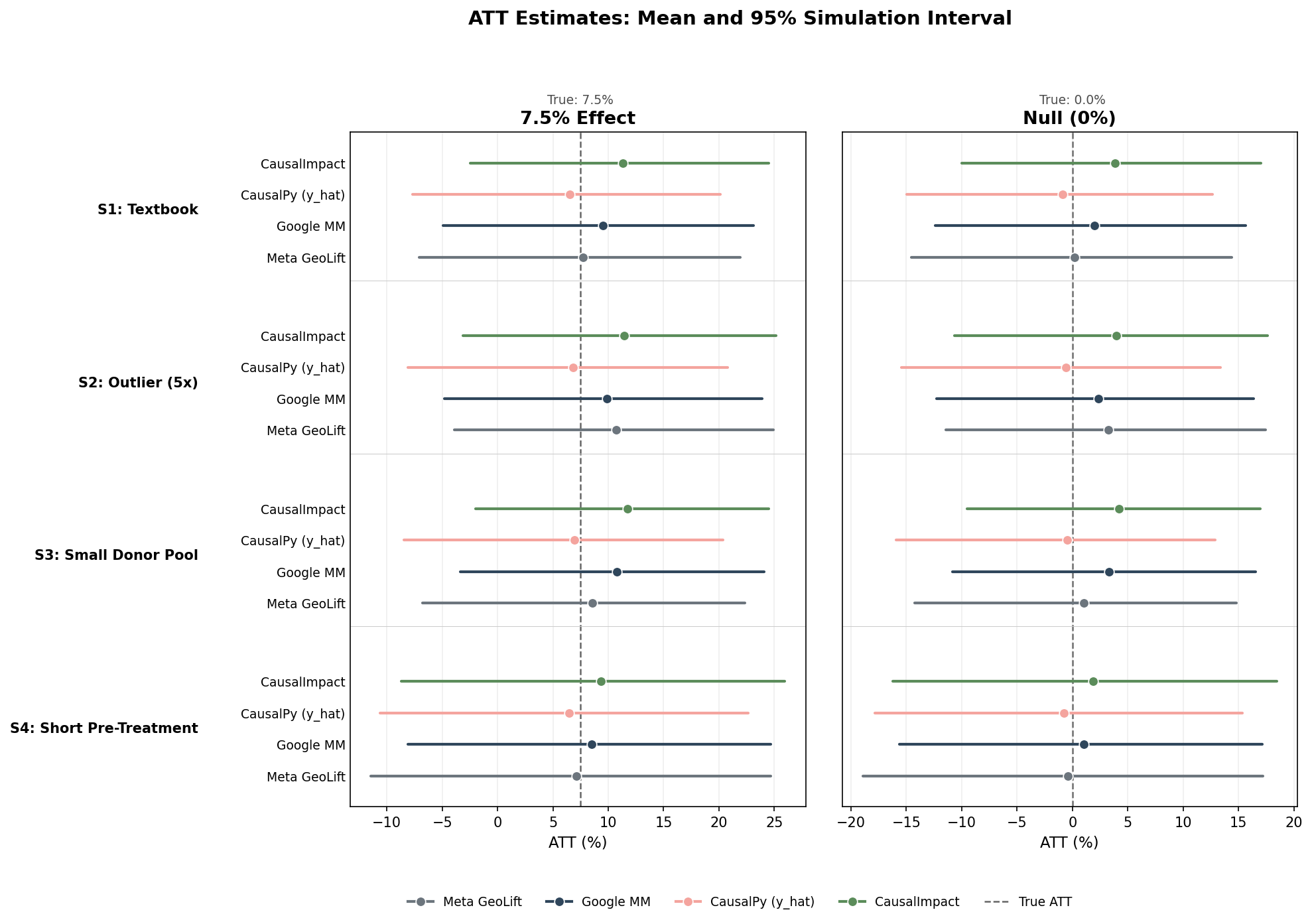
The exception is CausalPy in the outlier scenario (S2), where a data-scaling mismatch produces a near-6× overstatement out of the box (corrected to 6.81% after rescaling — see the Appendix for details). The outlier scenario inflates bias for every tool, but the magnitudes elsewhere stay within a few percentage points of the true lift.
Point estimates alone would tell you these tools are interchangeable. The uncertainty story tells you why they aren't.
Meta GeoLift produces the most honest confidence intervals of any tool tested — its stated ranges contain the true effect 92–95% of the time, and it almost never declares a winner that isn't real (false positive rate of 3–5%). The cost is that its intervals are very wide which can make decision-making more difficult. Even though its confidence intervals contain the true 7.5% effect 92–95% of the time, those intervals are wide enough that they also contain zero, and as a result, the test comes back inconclusive in 89% of baseline runs. This makes Meta GeoLift an appropriate choice when scaling budget behind a channel that doesn't actually work — the false positive — is more expensive for your business than missing a real, winning channel.
Google Matched Markets sits in the middle. It gives up some calibration (81–86% coverage) in exchange for more decisive results, with a false positive rate of 14–19% and a tendency to overestimate lift by 1–3 percentage points. When you need experiments to produce actionable answers and can tolerate a higher rate of false alarms, Google MM is a practical default.
CausalPy requires rescaling the input data before fitting1 — without it, its confidence intervals are far too narrow and its estimates unreliable, particularly when the treated market is much larger than the control markets. With rescaling, it lands in a similar range to Google MM on most metrics. Causal Impact consistently overestimates lift by 2–4 percentage points and has the worst coverage of any tool tested (70–72%). If you are currently using either tool, confirm your results hold up against known ground truth before relying on them for budget decisions — and for CausalPy specifically, ensure your pipeline rescales the data first.
"No tool fully compensates for a poorly designed experiment. When the treated market is dramatically larger than the control markets (the New York problem) confidence intervals across all four tools widen 4–5× and most tools overestimate lift by 2–4 percentage points. At that point, the choice of tool matters less than the choice of test market."
All simulation code, panel generation infrastructure, and analysis scripts are publicly available. The repository includes scripts to generate panels for all four scenarios, wrapper code for each tool, orchestration for parallel execution with checkpointing, and analysis code for every metric, table, and figure in this study.
We built this study to be extended. Change the scenarios, adjust tool configurations, add an estimator, plug in your own data. If you find results that differ from ours, we want to hear about it.
Every simulation study is only as good as the assumptions baked into it, and ours are no exception. Our synthetic data was designed to behave like real marketing data, but real geo-experiments add complications we didn't model — markets that move together due to national events, extreme outliers, spillover effects between neighboring cities, and so on.
It's also worth noting that some of GeoLift's strong performance in this study may reflect that our data was built in a way that happens to suit its statistical approach; under messier real-world conditions, the tool rankings could shift. Full details on these limitations are in the Appendix.
This is the first study in a series. Upcoming posts will include deep dives into each individual tool, simulations under more realistic and difficult data conditions, and eventually tests on real campaign data where the true answer isn't known in advance. If the rankings change under harder conditions, we'll report that too.
We recommend running the simulation yourself under different conditions and seeing if the findings hold.
Full methodology, fair-comparison protocol, scenario-by-scenario results, and configuration details for the 32,000-model-fit benchmark. For the narrative report, see the Executive Report.
We benchmark four open-source geo-experiment estimation tools — CausalPy, Google Matched Markets (MM), Meta GeoLift, and Causal Impact — on synthetic panels where the true treatment effect is known. Each scenario represents an operating condition practitioners encounter: ideal conditions; an outlier treated market; a small donor pool; and a short pre-treatment window. Each tool was run under two effect conditions (7.5% lift and 0% lift).
The central finding is that no tool delivers nominal 95% coverage while reliably detecting real incremental effects. At the extremes, Causal Impact detects most real lifts (FNR 34–48%) but fires on noise nearly a third of the time (FPR 28–30%); GeoLift holds false positives near nominal (FPR 3–5%) but misses 89–96% of real effects. The two middle tools, Google MM and CausalPy, are under-calibrated and, relative to Causal Impact, under-powered.
CausalPy required data standardization to produce proper uncertainty intervals. Without it, coverage ranged from 0.3% to 14.1% and false positive rate reached at least 86% across all scenarios; standardization lifted coverage to 76–82% and cut FPR to 18–25%.
Comparing tools that differ in statistical model, inference mechanism, and output format requires deliberate equalization. We standardized every dimension that is not an intrinsic property of the estimator, so that observed differences in performance reflect genuine estimator behavior rather than configuration choices.
| Dimension | Rule |
|---|---|
| Uncertainty level | 95% across all tools |
| Treated / control assignment | Identical per scenario (same panel files) |
| Pre / post split | Identical per scenario |
| True ATT% (benchmark) | Computed from DGP counterfactual, same for all tools |
| Tool ATT% and CI | Each tool reports its own estimate and interval |
| Bias | ATT% minus true ATT%, where true ATT% is either 7.5% or 0% |
| Significance criterion | 95% uncertainty interval excluding zero |
| False Positive Rate (FPR) | Share of null iterations where tool declares significance |
| False Negative Rate (FNR) | Share of effect iterations where tool fails to detect |
This protocol isolates three estimator-level differences:
The simulation study follows a factorial design: four market scenarios × two effect conditions (null effect or 7.5% effect) × 1,000 synthetic panel iterations = 8,000 unique datasets, each evaluated by all four tools (32,000 total model fits). All tools received identical panel files; no tool saw the true treatment effect. Each tool's output was recorded and evaluated against the known DGP ground truth.
Each synthetic panel is generated from a multiplicative model. For geo i at time t:
Y_cf(i,t) = baseline_i × trend_t × season_t × exp(noise_level × scale_i × ar_noise(i,t))
Where:
Treatment is multiplicative: Y_obs(i,t) = Y_cf(i,t) × (1 + τ) for post-period observations of the treated geo, where τ = 0 (null, 0% lift) or 0.075 (7.5% positive lift). The treated unit is the geo closest to the median baseline, ensuring it is representative of the control pool rather than an outlier — except in Scenario S2, where a 5× baseline inflation is applied to deliberately induce scale mismatch.
Key design choices: shared trend and seasonality ensure some cross-geo correlations. Multiplicative noise ensures Y is strictly positive and that noise variance scales with the geo's baseline — a common feature of sales and impression data.
CausalPy bakes in an assumption about how noisy your data should be before looking at it. Its default prior on observation noise, HalfNormal(sigma=1), works fine for small-scale KPIs like click-through rates. But daily revenue can swing by hundreds or thousands between cities and days, so the prior is far too tight for this application. As a result, practitioners would get distorted posteriors with confidence intervals that are narrow and overconfident in the wrong regions.
We identified two fixes. You may import pymc_extras and pass a custom sigma prior via PyMC's Prior object — but this requires navigating undocumented guidance on CausalPy's nested prior structure, and it still fails in S2 where the outlier geo runs at roughly 5× baseline. Or you may rescale (e.g. standardize) the input data before fitting. Rescaling solves both problems: it makes S2 viable for standard synthetic control and brings all series to unit variance, which is exactly what the default prior assumes.
We adopted rescaling after discussion with our research team. For each scenario, we standardized each geo's series against its pre-period mean and standard deviation before fitting, then converted estimates back to the original scale afterward. We discuss results both ways below — unscaled and scaled — because the unscaled version is what most practitioners will encounter first. We've also opened a pull request to the CausalPy repository to surface this requirement in their documentation.
For each geo independently, using only the days before treatment starts, we compute the pre-period mean and standard deviation. Every day's value is then replaced with (value − mean) / std. CausalPy runs on the rescaled data. Afterward, we undo the rescaling: the estimated treatment effect on rescaled units is multiplied by the treated geo's pre-treatment standard deviation to convert back to the original scale.
Standardization resolves the S2 outlier blowup and widens intervals approximately 5–10× , improving coverage from 0.3–14% to the 76–82% range observed in our final results. In the rest of this appendix, we contrast some results obtained without standardization to illustrate the magnitude of the problem.
Specific before/after numbers: in S1, coverage went from 13.4% to 80.3% and FPR from 86.6% to 19.8%; CI widths widened roughly 8× (from 95.42 to 749.10 daily-level units). In S2, ATT fell from 45.2% (bias +37.7 pp) to 6.81% (bias −0.69 pp), coverage rose from 0.3% to 82.1%, and FPR dropped from 99.7% to 18.2%. The pattern held across all scenarios, with CI widths widening 8–13×.
Per-scenario results follow, with each scenario's table, key observations, and the impact of CausalPy standardization. Figures 2 and 3 at the end of this section visualize ATT estimates and per-iteration uncertainty intervals across all conditions.
| Tool | Avg ATT (%) | Bias (pp) | Coverage | FNR | FPR | Avg CI Width |
|---|---|---|---|---|---|---|
| CausalPy (y_hat) | 6.50 | −1.00 | 80.30% | 66.20% | 19.80% (avg lift: −0.90%) | 749.10 |
| Google MM | 9.51 | +2.01 | 83.10% | 57.10% | 16.90% (avg lift: +2.01%) | 833.48 |
| Meta GeoLift | 7.72 | +0.22 | 92.20% | 91.30% | 4.60% (avg lift: +0.22%) | 2,020.07 |
| Causal Impact | 11.32 | +3.82 | 72.20% | 37.90% | 27.80% (avg lift: +3.82%) | 694.26 |
Even under ideal conditions, no tool hits nominal 95% coverage. GeoLift comes closest (92.20%) but at the cost of extremely wide intervals that make it nearly unable to detect a 7.5% effect (FNR = 91.30%). Causal Impact has the most detection power (FNR = 37.90%) but the worst false positive rate (FPR = 27.80%) and the largest bias (+3.82 pp).
Before standardization, CausalPy told a very different story in S1: 13.4% coverage, 8.0% FNR, 86.6% FPR, and CI width of just 95.42 units — a profile of extreme overconfidence. Standardization widened intervals roughly 8× (to 749.10 units), lifting coverage to 80.3% but shifting FNR from 8.0% to 66.2%. The trade-off is stark: proper calibration came at the cost of the ability to detect real effects.
| Tool | Avg ATT (%) | Bias (pp) | Coverage | FNR | FPR | Avg CI Width |
|---|---|---|---|---|---|---|
| CausalPy (y_hat) | 6.81 | −0.69 | 82.10% | 64.30% | 18.20% (avg lift: −0.59%) | 3,752.54 |
| Google MM | 9.85 | +2.35 | 81.70% | 53.00% | 18.30% (avg lift: +2.35%) | 4,170.03 |
| Meta GeoLift | 10.72 | +3.22 | 93.60% | 91.00% | 4.20% (avg lift: +3.22%) | 9,954.52 |
| Causal Impact | 11.46 | +3.96 | 70.00% | 37.20% | 30.00% (avg lift: +3.96%) | 3,489.26 |
The 5× outlier has minimal impact on relative tool ordering. All tools absorb the scale change through proportionally wider CIs. GeoLift's bias increases to +3.22 pp (from +0.22 in S1), suggesting the augmented synthetic control method picks up some of the outlier's scale. CausalPy remains the least biased.
This was not the case before standardization. Without it, CausalPy catastrophically failed in S2: ATT of 45.2% (bias +37.7 pp vs the true 7.5%), coverage of 0.3%, and FPR of 99.7%. The outlier's scale overwhelmed the default prior, producing wildly inflated estimates and near-zero-width intervals. Standardization resolved this entirely — ATT fell to 6.81%, coverage rose to 82.1%, FPR dropped to 18.2%.
| Tool | Avg ATT (%) | Bias (pp) | Coverage | FNR | FPR | Avg CI Width |
|---|---|---|---|---|---|---|
| CausalPy (y_hat) | 6.93 | −0.57 | 82.40% | 65.20% | 18.00% (avg lift: −0.46%) | 773.73 |
| Google MM | 10.80 | +3.30 | 80.90% | 47.30% | 19.10% (avg lift: +3.30%) | 828.80 |
| Meta GeoLift | 8.53 | +1.03 | 92.50% | 89.30% | 4.90% (avg lift: +1.03%) | 1,926.35 |
| Causal Impact | 11.71 | +4.21 | 71.10% | 34.30% | 28.90% (avg lift: +4.21%) | 686.57 |
Halving the donor pool from 20 to 9 barely changes the picture. This is expected: the DGP generates geos with shared trend and seasonality, so even a small pool provides adequate counterfactual donors. Google MM's bias worsens to +3.30 pp, the largest degradation of any tool in this scenario.
CausalPy's pre-standardization S3 profile mirrored S1: 14.1% coverage, 86.0% FPR, CI width of 93.91 units. After standardization, coverage improved to 82.4% and FPR fell to 18.0% — confirming that donor pool size was not the binding constraint; prior calibration was.
| Tool | Avg ATT (%) | Bias (pp) | Coverage | FNR | FPR | Avg CI Width |
|---|---|---|---|---|---|---|
| CausalPy (y_hat) | 6.45 | −1.05 | 75.90% | 63.50% | 24.80% (avg lift: −0.79%) | 718.74 |
| Google MM | 8.53 | +1.03 | 85.50% | 65.90% | 14.50% (avg lift: +1.03%) | 915.14 |
| Meta GeoLift | 7.11 | −0.39 | 95.10% | 95.70% | 3.30% (avg lift: −0.39%) | 5,574.99 |
| Causal Impact | 9.37 | +1.87 | 70.50% | 47.80% | 29.50% (avg lift: +1.87%) | 694.78 |
Cutting the pre-period from 90 to 30 days is the most disruptive scenario. CausalPy's coverage drops to 75.90% and its FPR rises to 24.80% — a meaningful degradation from S1. Google MM improves on bias (+1.03 pp, down from +2.01 in S1) and achieves its best FPR (14.50%) across all scenarios, suggesting TBR benefits from a tighter calibration window. GeoLift hits nominal coverage (95.10%) but almost never detects a real effect — its FNR reaches 95.70%, meaning it detects the effect fewer than 5 times in 100.
Before standardization, CausalPy's S4 profile was equally dire: 9.3% coverage, 90.6% FPR, CI width of 82.42 units. Standardization brought coverage to 75.9% and FPR to 24.8% — the weakest post-standardization results across scenarios, confirming that shorter pre-periods compound the difficulty of prior calibration.
In the left panel in figures 2.A and 2.B (effect condition), CausalPy centers closest to the true 7.5% but with a slight negative bias. Causal Impact consistently overshoots. GeoLift's simulation intervals are the widest, consistent with its conservative conformal inference. In the right panel (null condition), a well-calibrated tool should center on zero with intervals that rarely exclude it. Causal Impact's mean drifts +1.87 to +4.21 pp above zero across all scenarios — the same positive bias that inflates its false positive rate.
GeoLift's columns are almost entirely green (92–95%), confirming its conservative calibration. Causal Impact shows heavy red, especially in S2 and S4 — roughly 30% of its credible intervals miss the truth under the outlier and short pre-treatment scenarios. CausalPy and Google MM fall in between, with coverage in the 76–86% range.
Every simulation study has blind spots. Here are ours:
| Tool / Package | Version | Source |
|---|---|---|
| CausalPy | 0.8.0 | PyPI |
| PyMC | 5.28.1 | PyPI |
| ArviZ | 0.23.4 | PyPI |
| Google matched_markets | commit 5e3cd95 | GitHub |
| Meta GeoLift | v2.7.5 / commit 4d2afd4 | GitHub |
| augsynth | commit 65c5a6f | GitHub |
| Causal Impact | 1.4.1 | CRAN |
| Python | 3.12.8 | — |
| Parameter | CausalPy | Google MM | GeoLift | Causal Impact |
|---|---|---|---|---|
| Confidence | 95% HDI | 95% CI | alpha = 0.05 | alpha = 0.05 |
| MCMC | 4 chains × 1,000 + 1,000 warmup | — | — | 2,000 iter |
| Seasonality | — | — | — | nseasons=7, duration=1 |
| Model | Dirichlet SC | OLS TBR | Ridge ASCM | BSTS local level |
| Inference | HDI | t-distribution | conformal (block) | Bayesian credible |
| Parameter | Value |
|---|---|
| Geos (default) | 1 treated + 20 control |
| Total days (default) | 105 (90 pre + 15 post) |
| Baseline mean | 4,000 |
| Baseline spread (sdlog) | 0.6 |
| Trend slope | 0.001/day (0.1%) |
| Seasonality amplitude | 0.10 |
| DOW profile (Mon–Sun) | [−1.0, −0.5, 0.0, 0.2, 0.8, 1.0, 0.5] |
| AR(1) coefficient | 0.30 |
| Noise level (log-scale) | 0.20 |
| Outlier multiplier (S2) | 5.0 |
| Iterations per cell | 1,000 |
| Master seed | 42 |
| Path | Description |
|---|---|
| config/tools.yaml | Tool configurations |
| src/R/generate_panels.R | Data-generating process |
| src/R/run_geolift.R | GeoLift wrapper |
| src/R/run_causalimpact.R | Causal Impact wrapper |
| src/python/run_causalpy.py | CausalPy wrapper |
| src/python/run_google_mm.py | Google MM wrapper |
| analysis/compute_metrics.py | Metric aggregation |
| analysis/generate_tables.py | Table generation |
| analysis/plot_forest.py | ATT forest plot |
| analysis/plot_ci_gallery.py | CI gallery figure |
| results/aggregated/ | Final tables and metrics |
| results/raw/results.jsonl | Raw per-iteration results |
| panels/ | Generated synthetic data (parquet) |
| figures/ | All figures |
One email when the next study in this series is published. Nothing else.
Something went wrong — please try again.
The Marketing Measurement Roundup — the best of marketing measurement, every week.
Something went wrong — please try again.